Ola Sanusi, PhD

Educator | Data Scientist | Researcher
View My LinkedIn Profile
| Predicting Baltimore City (MD) Crimes using SARIMAX and fbProphet model | Time Series Forecasting Author: Ola Sanusi, PhD |
Introduction
This project involves using (S)ARIMA(X) and fbProphet to predict Baltimore City crimes. The goal is to use historical Baltimore City, MD data obtained from Baltimore Open Data Website to forecast crimes so that the Police Department will be able to allocate appropriate resources to the right neighborhood and district. The project is two fold (1) identify the most important crimes that need special attention (2) utlize both the (S)ARIMA(X) and fbProphet time series models to predict the monthly crime rates for important crimes by resampling the data to cover long term (months ahead) forecasting using (S)ARIMA(X) and fbProphet.
The crime data covering a 7 year period (Jan 1, 2014 — Dec 31, 2020) was be used in predicting the crime rates for different crime types occuring in Baltimore. The objective is to predict the crimes for the next 2 years.
The Dataset
The Baltimore City crime data consist of all crime types that occur between October 1963 and March 2021. Data preprocessing performed involves removing all columns that has over 70% missing values, dropping unneeded columns, filling remaining missing values with the mode of each categorical variables.
| CrimeDateTime | Location | Description | District | Neighborhood | Latitude | Longitude | GeoLocation | |
|---|---|---|---|---|---|---|---|---|
| 0 | 2021/03/25 01:20:20+00 | 0 S CAREY ST | HOMICIDE | SOUTHERN | UNION SQUARE | 39.2879 | -76.6382 | (39.2879,-76.6382) |
| 1 | 2021/03/25 01:20:20+00 | 0 S CAREY ST | SHOOTING | SOUTHERN | UNION SQUARE | 39.2879 | -76.6382 | (39.2879,-76.6382) |
| 2 | 2021/03/24 00:08:00+00 | 4900 YORK RD | COMMON ASSAULT | NORTHERN | WINSTON-GOVANS | 39.3480 | -76.6096 | (39.348,-76.6096) |
| 3 | 2021/03/24 07:53:00+00 | 400 E PATAPSCO AVE | COMMON ASSAULT | SOUTHERN | BROOKLYN | 39.2372 | -76.6049 | (39.2372,-76.6049) |
| 4 | 2021/03/24 21:54:00+00 | 2500 GREENMOUNT AVE | ROBBERY - CARJACKING | NORTHERN | HARWOOD | 39.3182 | -76.6095 | (39.3182,-76.6095) |
From the raw dataset, data from 1963 to 2013 is very sparse with just few data recorded per year. Therefore, for this project, the dataset was subsetted from 2014 to 2020 which covers 7 years period.
bpd = bpd[(bpd['year']>=2014) & (bpd['year']!=2021)]
Finally, the crime date was converted to pandas datetime with the index as datetimeindex.
Exploratory Data Analysis (EDA)
Descriptive statistics
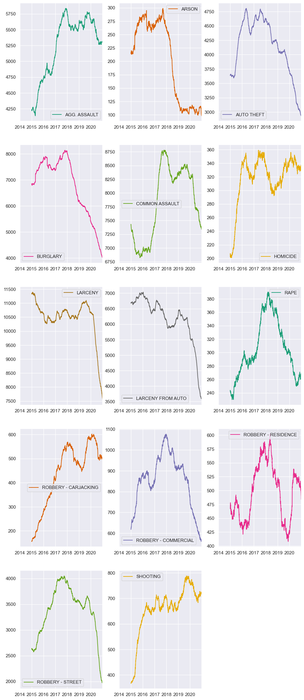
If you look at the trend for each of the crime types from the above reported crime type trend, only three (homicide, robbery-carjacking and shooting) are showing an increasing trend. The others reveals somewhat decreasing trends from the previous years.
In lieu of this findings, time series forecasting was used to model trends for the following:
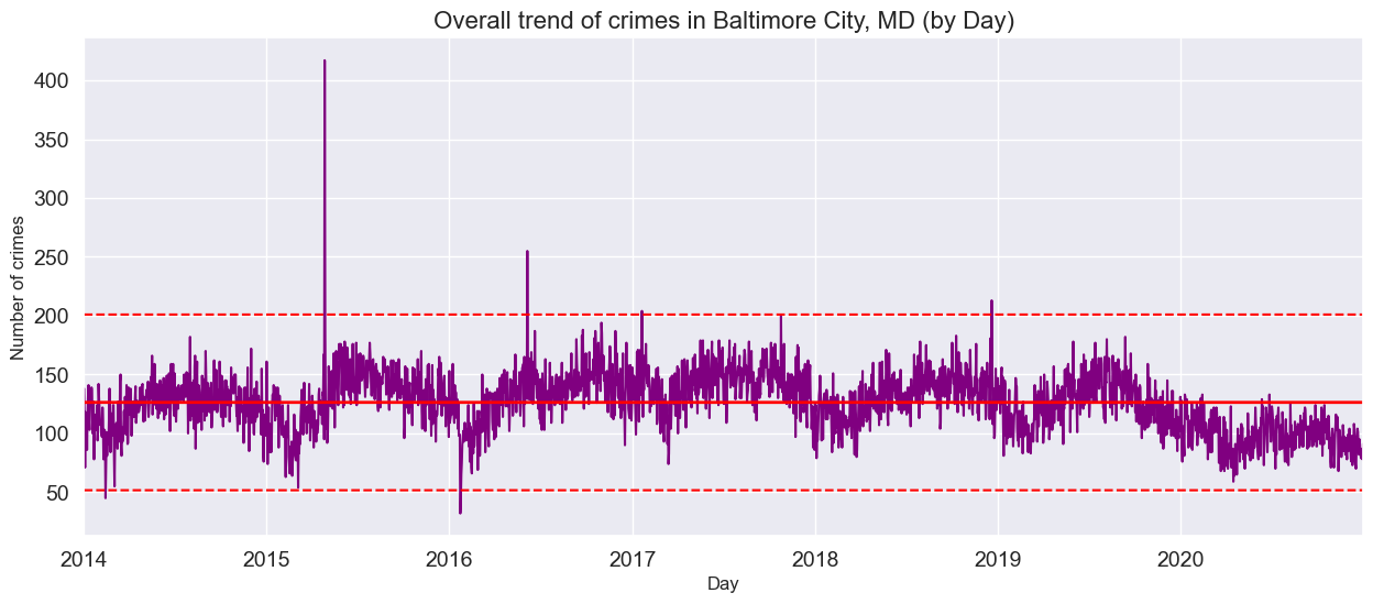
- Overall crimes occuring irrespective of types
- All crime types showing increasing trend
- homicide
- robbery-carjacking
- shooting
- Crime types showing decreasing trend
- rape
- agg.assault
Building new dataframes for the Time Series model
## In order to analyze the specific crime types, new dataframes for the specific crimes are built.
crime=bpd.copy()
homicide = crime[crime['Description']=='HOMICIDE']
rape = crime[crime['Description']=="RAPE"]
shooting = crime[crime['Description']== "SHOOTING"]
carjack = crime[crime['Description']=="ROBBERY - CARJACKING"]
assault = crime[crime['Description']=="AGG. ASSAULT"]
Time-series seasonal decomposition
def decompose_dataframe(df):
    y = df.resample ('MS').size ()
    decomposition = sm.tsa.seasonal_decompose(y, model='additive')
    fig = decomposition.plot()
    fig.set_figheight(8)
    plt.show()
decompose_dataframe(crime)
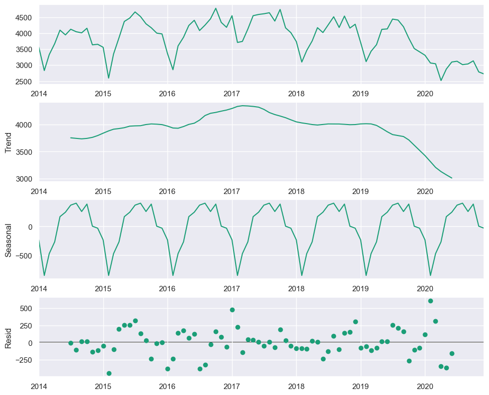
The overall crime trend reveals that crimes start increasing gradually from 2014 until it reached the peak in 2017 and start decreasing steadily until reaching the lowest in 2020
Using Pyramid Arima to determine the optimal SARIMAX parameters
#Split dataset to train and test using sktime
y_train, y_test = temporal_train_test_split(resampled(crime), test_size=24)
plot_series(y_train, y_test, labels=["y_train", "y_test"])
print(y_train.shape[0], y_test.shape[0])
from pmdarima.arima import auto_arima
sarimax_model = auto_arima(y_train, start_p=1, d=1, start_q=1, max_p=8, max_d=2, max_q=8,
                        start_P=0, D=None, start_Q=0, max_P=8, max_D=1, max_Q=8,
                        m=12, seasonal=True, stationary=False,
                        information_criterion='aic', alpha=0.05, test='kpss',
                        seasonal_test='ocsb', stepwise=True, n_jobs=-1,
                        start_params=None, trend=None, method='lbfgs',
                        maxiter=50, offset_test_args=None, seasonal_test_args=None,
                        suppress_warnings=True, error_action='warn', trace=False,
                        random=False, random_state=500, n_fits=30)
| Dep. Variable: | y | No. Observations: | 60 |
|---|---|---|---|
| Model: | SARIMAX(2, 1, 0)x(1, 0, [1], 12) | Log Likelihood | -411.837 |
| Date: | Sat, 07 Aug 2021 | AIC | 835.673 |
| Time: | 09:21:19 | BIC | 848.138 |
| Sample: | 0 | HQIC | 840.539 |
| - 60 | |||
| Covariance Type: | opg |
Fitting the SARIMAX model
mod = sm.tsa.statespace.SARIMAX(y_train,
                                order=(2, 1, 0),
                                seasonal_order=(1, 0, 1, 12),
                                enforce_stationarity=False,
                                enforce_invertibility=False)
results = mod.fit()
#Diagnosing the model residuals
results.plot_diagnostics(figsize=(15,12))
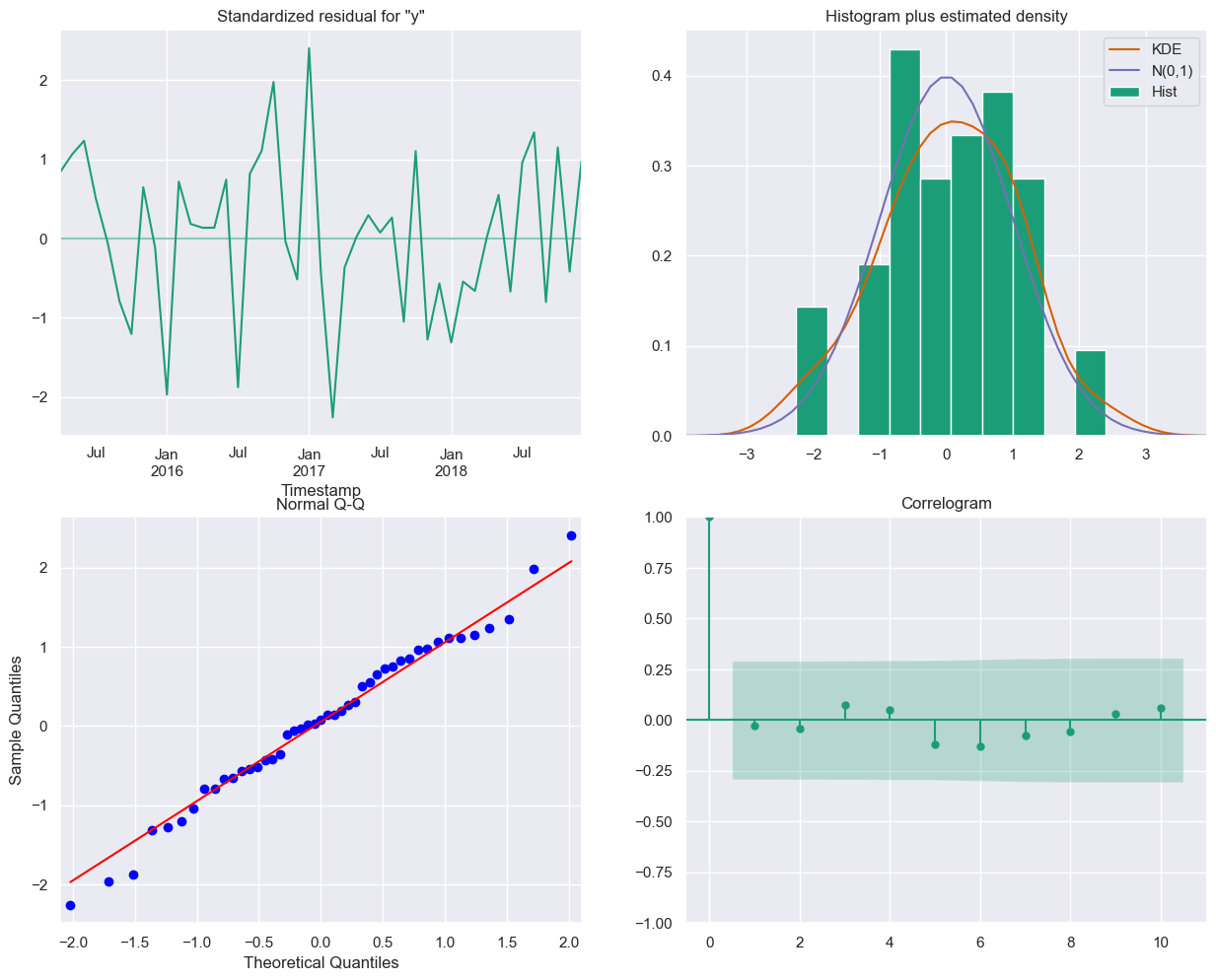
Modeling with SARIMAX
Overall crime forecasting in Baltimore city, MD
%%time
# Predictions on test set.

# Setting dynamic = True so that the model won't use actual values for prediction. Basically the model will use
# the lag terms and moving average terms of the already forecasted values. So, we will see the errors
#(confidence interval) increasing with each forecast.
#Forecasting 2 years steps ahead
pred = results.get_prediction(start=y_test.index[0], end=y_test.index[-1],
                              dynamic=True)

#Confidence intervals of the forecasted values
pred_ci = pred.conf_int()

#Plot the data
ax = y_train.plot(figsize = (14, 7), label='overall crime count', legend = True, color='g')
y_test.plot(ax=ax, label='Observed crime count', figsize= (14,7), color='g')
#Plot the forecasted values
pred.predicted_mean.plot(ax=ax, label='Forecasts crime count', figsize = (14, 7), alpha=.7, color='r')

#Plot the confidence intervals
ax.fill_between(pred_ci.index,
                pred_ci.iloc[:, 0],
                pred_ci.iloc[:, 1], color='k', alpha=.2)

plt.title('Overall Crime - Baltimore, MD', size = 16)
plt.ylabel('Count', size=12)
plt.xlabel('Date', size=12)
plt.legend(loc='upper center', prop={'size': 12})

plt.show()
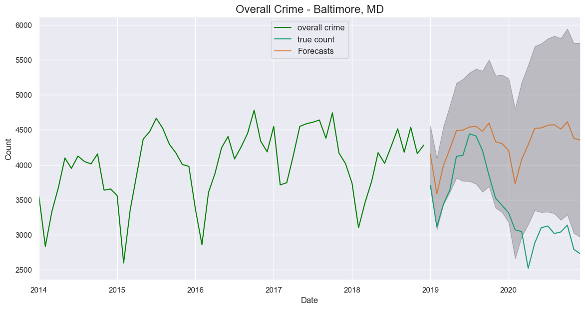
The SARIMAX model prediction was way off the observed crime count. Therefore, fbProphet which is a more powerful time series package was used.
Modeling with fbProphet
%%time
from fbprophet import Prophet
# Make the prophet model and fit on the data
dd_model = Prophet(interval_width=0.95)
dd_model.fit(ddf)
# Make a future dataframe for 3 years
dd_forecast = dd_model.make_future_dataframe(periods=24, freq='MS')
# Make predictions
dd_forecast = dd_model.predict(dd_forecast)
plt.figure(figsize=(15, 6))
dd_model.plot(dd_forecast, xlabel = 'Date', ylabel = 'Count')
plt.title('Overall Crime');
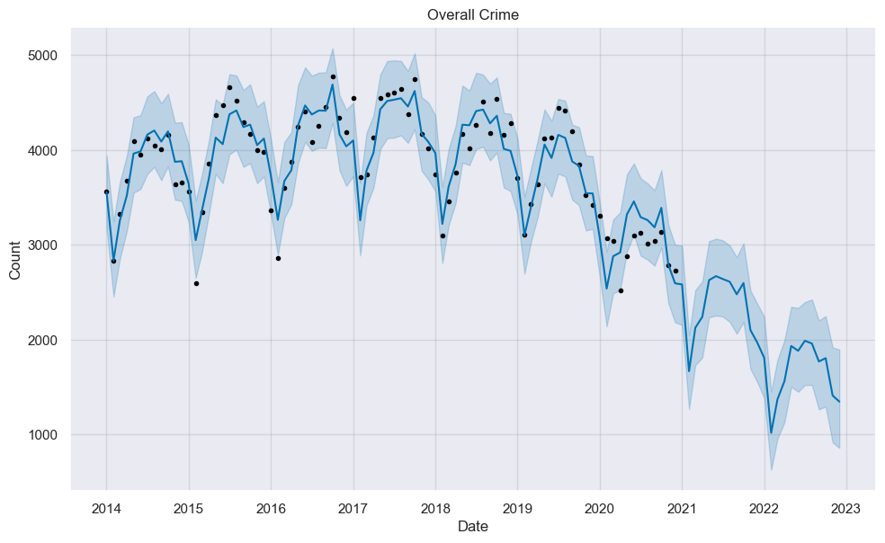
The black dots represent the actual values (notice how they stop at the end of 2020), the blue line indicates the forecasted values, and the light blue shaded region is the uncertainty (always a critical part of any prediction). The region of uncertainty increases the further out in the future the prediction is made because initial uncertainty propagates and grows over time. This is observed in crime forecasts which get less accurate the further out in time they are made.
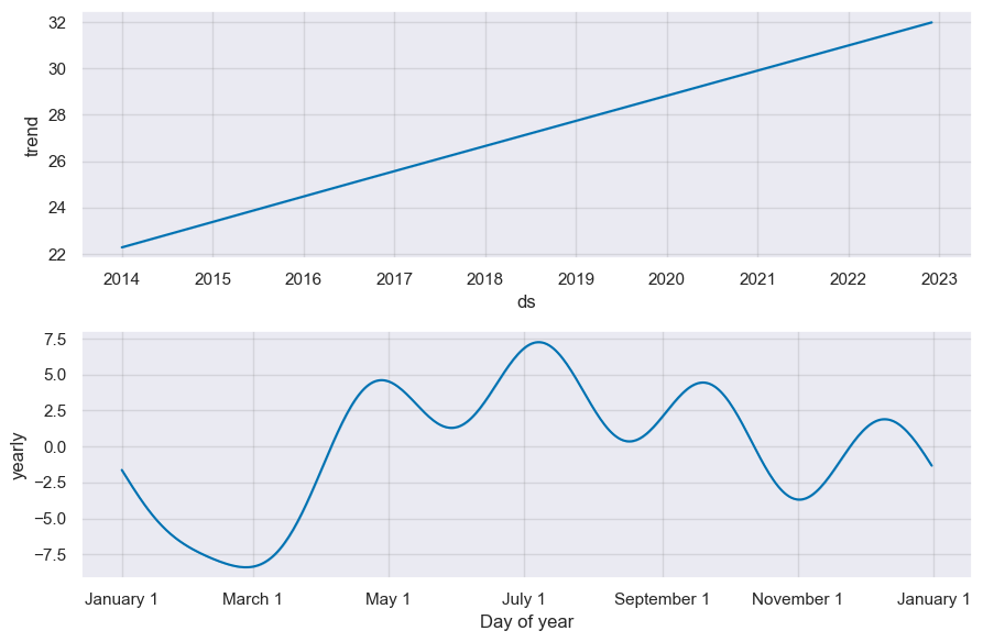
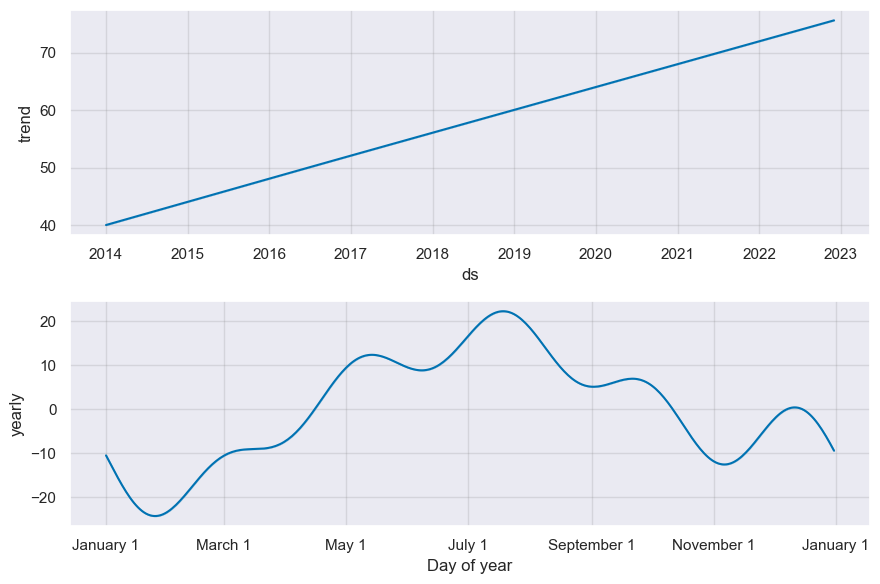
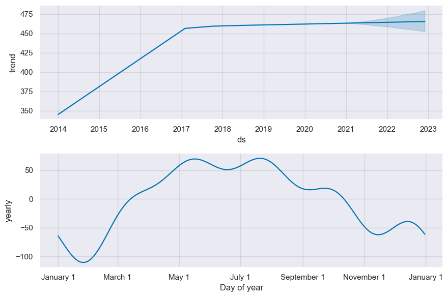
fbprophet component plot
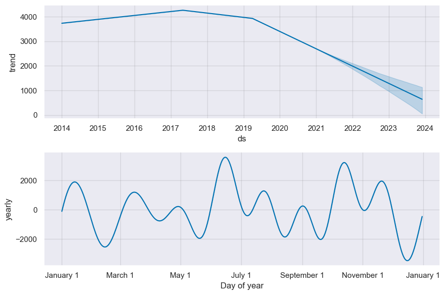
The result from the fbProphet prediction shows that the model fit perfectly which reveals the decreasing trend of the crime after 2017 which matches the decreased trend that occurs in the observed crime count.
fbProphet Forecasting trends for specific crime type
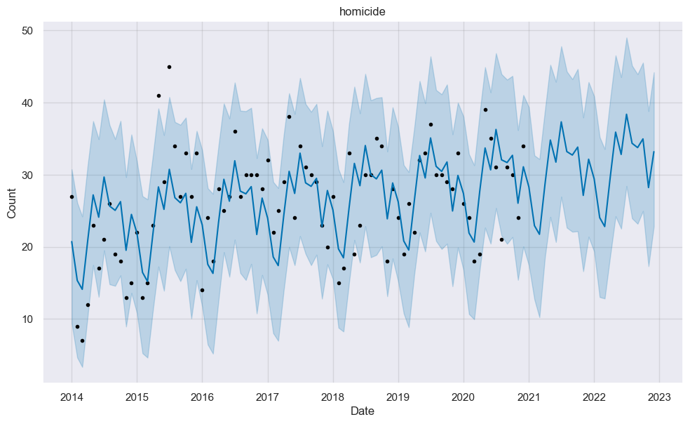
homicide
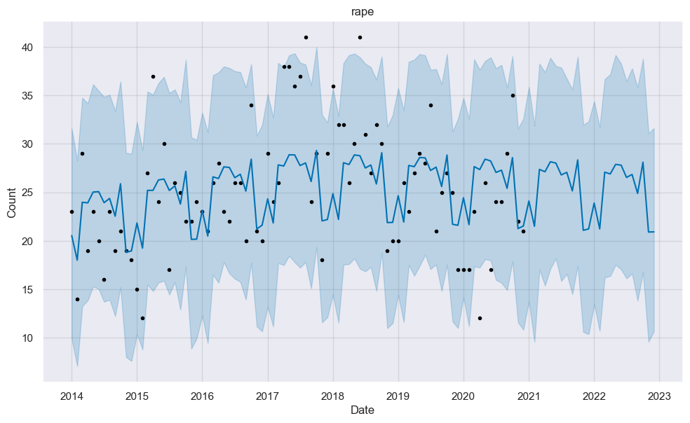
rape
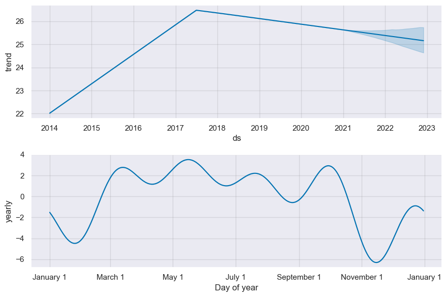
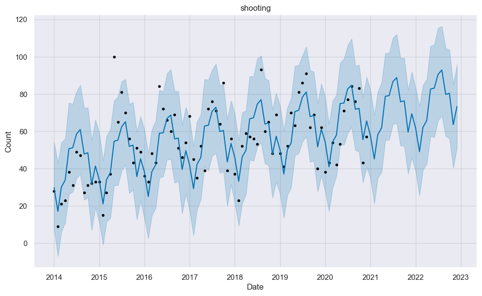
shooting
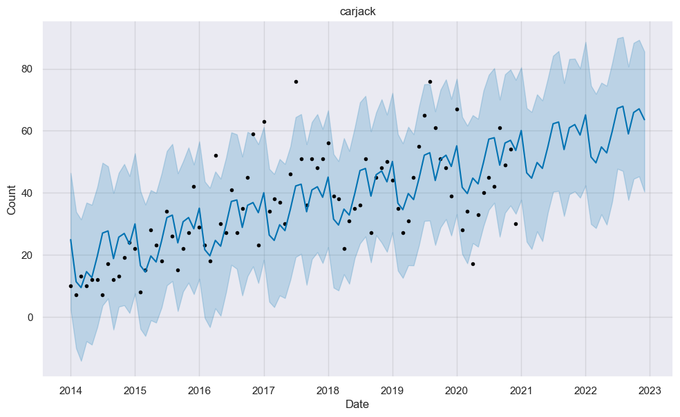
carjacking
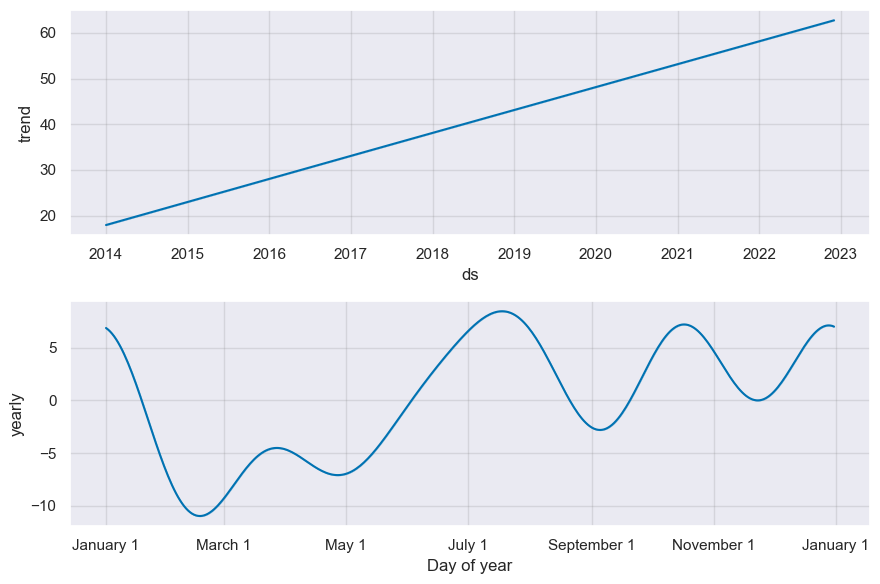
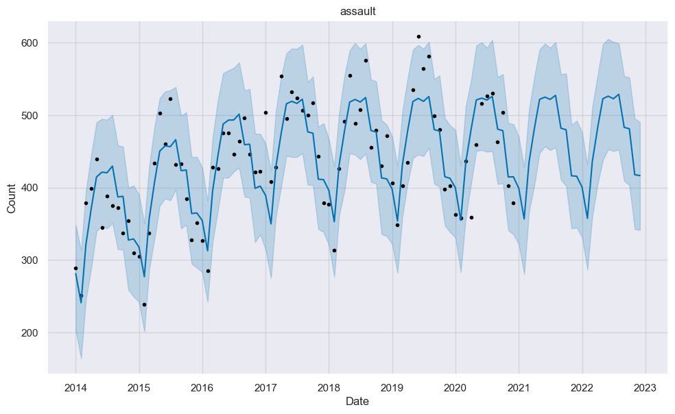
assault
| Crime Types | Forecasted trend |
|---|---|
| Agg. assault | constant/steady |
| Homicide | increasing |
| Rape | decreasing |
| Robbery-Carjacking | increasing |
| Shooting | increasing |
For each of the individual crime types investigated. The fbProphet model reveals a steady increasing trend for homicide with the highest crime count occurring in July. Homicide increased steadily with the highest crime count occuring during the summer (July) and the lowest around spring (March). The observed increasing trend will continue through 2023.
Shooting has a similar increasing trend as homicide which strongly suggest a correlation between the two crime types. The highest crime count also occurs in July with the lowest occurring around February/March.
Rape shows sharp increase from 2014 to the highest count in 2017 before beginning a gradual decreasing trend. This model reveals that rape which continue to decrease steadily. Most of reported rape cases is expected to occur between March and November will suggest warmer weather influence this crime type.
Carjacking is a crime of concern in Baltimore city because of the increasing trends and the fluctuating nature where the crime count goes up and down throughout the year. Highest carjacking is expected to occur around July, November and January.
Agg. assault increases steadily untill 2017 where the crime experiences the highest count. This crime type count will remain constant untill 2023.
Conclusion
In summary, the overall crime in Baltimore City, MD is projected to follow a decreasing trend, with the highest occurrences between May and October. On the other hand, homicide and shooting will increase steadily and agg. assaults remaining constant. The only crime type that shows a decreasing trend is rape.
Check out full codes and notebook on github